using Plots

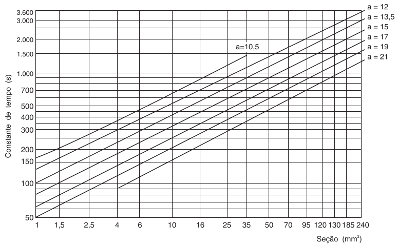
k_T = 300   # Constante de tempo de referência (s)
m = 2       # Relação de sobrecarga térmica de referência

n = range(sqrt(m) + 1e-3, 15, length=400)  # domínio válido: n² > m

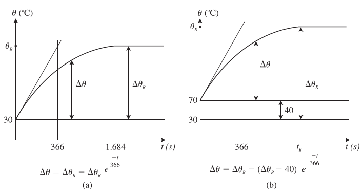
# Tempo até θ_S partindo a frio (Expressão 9.35)
t1 = @. k_T * log(n^2 / (n^2 - m))

# Tempo até θ_S partindo a quente (Expressão 9.36)
t2 = @. k_T * log((n^2 - 1) / (n^2 - m))

plt = plot(n, t1,
    label="Partida a frio (t₁)",
    linewidth=2,
    xlabel="Relação de sobrecarga n = I/Iz",
    ylabel="Tempo t (s)",
    title="Curvas de sobrecarga t = f(n)",
    xscale=:log10,
    yscale=:log10,
    xticks=([1, 1.5, 2, 3, 4, 5, 6, 7, 8, 9, 10, 15], ["1", "1,5", "2", "3", "4", "5", "6", "7", "8", "9", "10", "15"]),
    legend=:topright,
    size=(700, 420))

plot!(plt, n, t2, label="Partida a quente (t₂)", linewidth=2, linestyle=:dash)

# Ponto de exemplo citado no livro: n = 4
n_ex = 4
t1_ex = k_T * log(n_ex^2 / (n_ex^2 - m))
t2_ex = k_T * log((n_ex^2 - 1) / (n_ex^2 - m))
scatter!(plt, [n_ex, n_ex], [t1_ex, t2_ex], color=:red, label="n = 4 (exemplo do livro)")

println("Para n = 4: t1 (a frio) ≅ $(round(t1_ex, digits=1)) s, t2 (a quente) ≅ $(round(t2_ex, digits=1)) s")

display(plt)